Self-Attention from Scratch: The Heart of the Transformer
I’m writing this post mostly to make sure this stuff actually sticks in my head. Step-by-step explanations of self-attention with working examples are hard to find.
If you have used ChatGPT, Claude, or any modern language model, you have interacted with a Transformer. The Transformer is the architecture behind virtually every large language model (LLM) today. It was introduced in the legendary 2017 paper “Attention Is All You Need” by Vaswani et al. The entire architecture revolves around a single, elegant idea: self-attention.
Confession: I went in with all the confidence of someone holding a maths degree, and still failed to finish the paper! It is dense, and I ended up gathering the ideas from other sources.
In this post, I will build self-attention from scratch using PyTorch. I will start with a raw sentence, break it into tokens, turn those tokens into numbers, and then walk through — step by step — how self-attention computes a context-aware representation of each word.
What Problem Does Self-Attention Solve?
Consider the sentence:
“The cat sat on the warm mat”
As humans, we understand this sentence effortlessly. We know that “sat” is what the cat did, that “warm” describes the mat, and that “the” is just a grammatical particle. But a computer sees this as a sequence of symbols — it has no inherent understanding of relationships between words.
Traditional models like RNNs (Recurrent Neural Networks) process words one at a time, left to right. By the time the model reaches “mat”, its memory of “cat” has faded. Long-range dependencies are hard to capture.
Self-attention solves this. Instead of reading words sequentially, self-attention lets every word “look at” every other word in the sentence simultaneously. Each word can directly attend to every other word, regardless of how far apart they are, and decide how much each word matters in a given context.
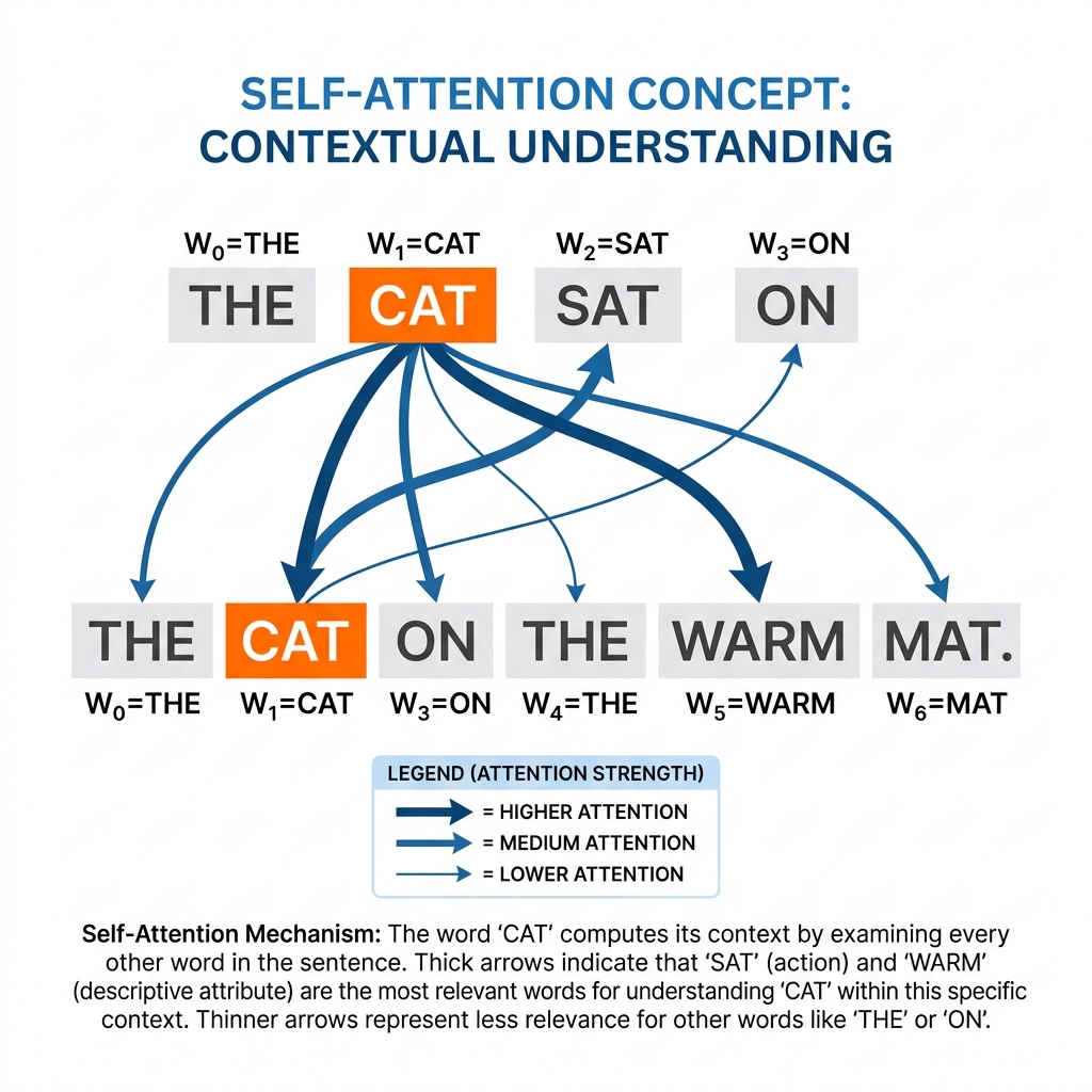
In the diagram above, the word “cat” is looking at all other words. The thicker the arrow, the more attention “cat” pays to that word. Notice how “cat” pays strong attention to “sat” (its action) and “warm” (which describes the surface it’s sitting on), but less attention to function words like “on” and “the”.
Where Does Self-Attention Fit in a Transformer?
Before diving into the math, let’s situate self-attention within the broader Transformer architecture.
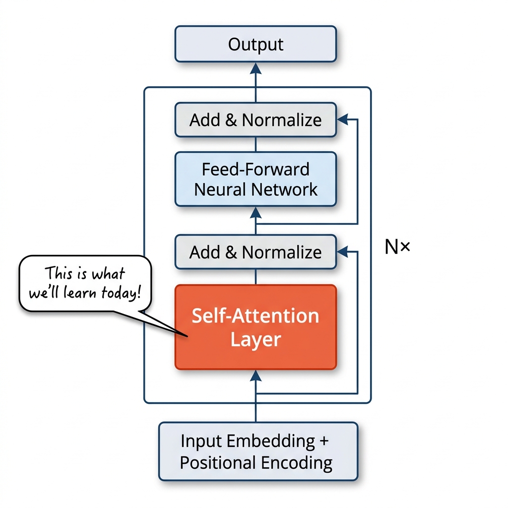
A Transformer is built from stacked layers, and each layer has two main sub-components:
- Self-Attention Layer — this is what we are building today
- Feed-Forward Neural Network — a standard dense network applied independently to each position
Each sub-component is followed by an Add & Normalize step (residual connections + layer normalisation). These layers are stacked $N$ times.
Today, we are focusing entirely on the Self-Attention Layer — the orange block in the diagram. Once you understand self-attention, the rest of the Transformer becomes much easier to grasp.
The Full Pipeline: From Raw Text to Context Vectors
Here is the complete journey we will walk through:
Raw Text → Tokenisation → Embedding → Attention Scores → Softmax → Context Vector
Let’s go step by step.
Step 1: Tokenisation
Our input is a raw string: "The cat sat on the warm mat".
The first thing any NLP model does is tokenise the input — break the sentence into individual units (tokens). For simplicity, we will use word-level tokenisation (each word becomes one token).
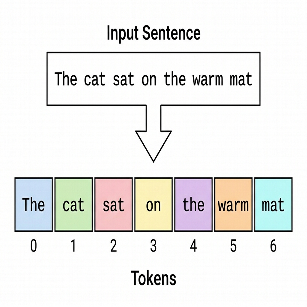
sentence = "The cat sat on the warm mat"
tokens = sentence.split()
print(tokens)
# ['The', 'cat', 'sat', 'on', 'the', 'warm', 'mat']
print(f"Number of tokens: {len(tokens)}")
# Number of tokens: 7
In real Transformer models (like GPT or BERT), tokenisation is more sophisticated — they use subword tokenisers like Byte-Pair Encoding (BPE) or WordPiece that split rare words into smaller pieces. But for learning self-attention, word-level tokenisation is perfectly fine.
Each token gets assigned a position index:
| Index | Token |
|---|---|
| 0 | The |
| 1 | cat |
| 2 | sat |
| 3 | on |
| 4 | the |
| 5 | warm |
| 6 | mat |
Step 2: Token Embedding
Computers cannot work with raw text directly. We need to convert each token into a numerical vector — a list of numbers that the model can process. This is called an embedding.
In a real model, embeddings are learned during training. Each word in the vocabulary gets its own vector, and similar words end up with similar vectors. For this tutorial, we will use small 3-dimensional vectors to keep things easy to follow.
import torch

# Each row is the embedding vector for one token
# In practice, these are learned — here we define them manually
inputs = torch.tensor(
    [[0.41, 0.12, 0.73],  # The   (x^1)
     [0.58, 0.91, 0.44],  # cat   (x^2)
     [0.33, 0.76, 0.89],  # sat   (x^3)
     [0.15, 0.42, 0.67],  # on    (x^4)
     [0.39, 0.14, 0.71],  # the   (x^5)
     [0.82, 0.53, 0.29],  # warm  (x^6)
     [0.61, 0.85, 0.47]]  # mat   (x^7)
)

print(f"Input shape: {inputs.shape}")
# Input shape: torch.Size([7, 3])
# 7 tokens, each represented by a 3-dimensional vector
So our input matrix is a $7 \times 3$ tensor — 7 tokens, each with a 3D embedding. We refer to each token’s embedding as $x^{(i)}$ where $i$ is the token position.
One thing to watch: the maths notation is 1-based ($x^{(1)}$ to $x^{(7)}$), but Python indexing is 0-based. So $x^{(2)}$, the embedding for “cat”, is inputs[1] in code.
Why Embeddings?
You might wonder: why not just use one-hot vectors (like [0, 0, 1, 0, 0, 0, 0] for “sat”)? Two reasons:
- Dense representation: One-hot vectors are sparse and high-dimensional. Embeddings are compact and dense.
- Semantic meaning: Embeddings are learned so that words with similar meanings have similar vectors. The distance between “cat” and “kitten” would be small, while the distance between “cat” and “algorithm” would be large.
Step 3: Computing Attention Scores (Dot Products)
Now comes the core of self-attention. The fundamental question is:
For a given token, how much should it “attend to” (pay attention to) each other token in the sequence?
To answer this, we compute attention scores. The simplest way to measure how related two tokens are is the dot product of their embedding vectors.
What is a Dot Product?
The dot product of two vectors $\mathbf{a} = [a_1, a_2, a_3]$ and $\mathbf{b} = [b_1, b_2, b_3]$ is:
$$\mathbf{a} \cdot \mathbf{b} = a_1 b_1 + a_2 b_2 + a_3 b_3$$
The dot product gives a single number (scalar) that measures how “aligned” two vectors are:
- Large positive value → vectors point in a similar direction → tokens are related
- Near zero → vectors are orthogonal → tokens are unrelated
- Negative value → vectors point in opposite directions
Choosing a Query Token
In self-attention, each token takes a turn being the query — the word that is asking, “Which other words should I pay attention to?” Every other token is a key that the query compares itself against.
Let’s pick "cat" (token at index 1) as our query:
# Select "cat" (index 1) as the query token
query = inputs[1]
print(f"Query (cat): {query}")
# Query (cat): tensor([0.58, 0.91, 0.44])
Now, we compute the dot product of the query with every token in the sequence (including itself):
# Compute attention scores for the query "cat" against all tokens
attn_scores_2 = torch.empty(inputs.shape[0])

for i, x_i in enumerate(inputs):
    attn_scores_2[i] = torch.dot(x_i, query)

print("Attention scores for 'cat':")
print(attn_scores_2)
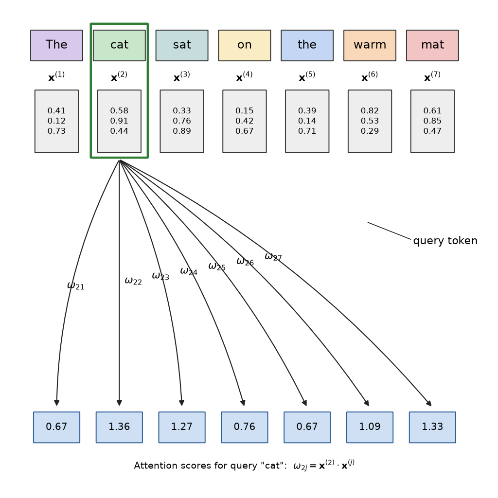
# tensor([0.6682, 1.3581, 1.2746, 0.7640, 0.6660, 1.0855, 1.3341])
Let’s break down what just happened. For each token $x^{(j)}$, we computed:
$$\omega_{2j} = x^{(2)} \cdot x^{(j)}$$
where $x^{(2)}$ is the embedding of “cat” (our query) and $x^{(j)}$ is the embedding of token $j$.
| Pair | Dot Product ($\omega$) | Meaning |
|---|---|---|
| cat · The | 0.6682 | low relevance |
| cat · cat | 1.3581 | highest (self-similarity) |
| cat · sat | 1.2746 | high relevance |
| cat · on | 0.7640 | low relevance |
| cat · the | 0.6660 | low relevance |
| cat · warm | 1.0855 | moderate relevance |
| cat · mat | 1.3341 | high relevance |
“cat” pays the most attention to itself (a vector’s dot product with itself is always high), followed closely by “mat” and “sat”. A caveat: I made these embedding values up, so any pattern here is a happy accident, not real semantics. In a trained model the embeddings are learned, and the attention pattern reflects genuine relationships between words.
We can also compute this much more efficiently using matrix multiplication instead of a for-loop:
# Efficient version using matrix-vector multiplication
attn_scores_2_efficient = inputs @ query
print(attn_scores_2_efficient)
# tensor([0.6682, 1.3581, 1.2746, 0.7640, 0.6660, 1.0855, 1.3341])
The @ operator performs matrix-vector multiplication, which computes all dot products in one step. This is exactly what real implementations use for speed.
Step 4: Normalising with Softmax (Computing Attention Weights)
The raw dot-product scores ($\omega$ values) are useful, but they have a problem: they can be any real number, and their magnitudes depend on the dimensionality of the embeddings. We need to normalise them so that:
- All weights are positive (negative attention doesn’t make sense)
- All weights sum to 1 (so they form a proper probability distribution)
This is exactly what the softmax function does.
What is Softmax?
The softmax function converts a vector of arbitrary real numbers into a probability distribution:
$$\text{softmax}(z_i) = \frac{e^{z_i}}{\sum_{j} e^{z_j}}$$
For a vector $\mathbf{z} = [z_1, z_2, \ldots, z_n]$:
- Each element is exponentiated ($e^{z_i}$), which makes it positive
- Then divided by the sum of all exponentiated values, which makes them sum to 1
- Larger input values get exponentially larger weights (softmax amplifies differences)
Applying Softmax Step by Step
Let’s apply softmax to our attention scores manually first:
# Step-by-step softmax calculation

# Step 1: Exponentiate each score
exp_scores = torch.exp(attn_scores_2)
print("Exponentiated scores:")
print(exp_scores)
# tensor([1.9507, 3.8888, 3.5773, 2.1468, 1.9464, 2.9609, 3.7966])

# Step 2: Sum all exponentiated scores
exp_sum = exp_scores.sum()
print(f"\nSum of exp scores: {exp_sum:.4f}")
# Sum of exp scores: 20.2676

# Step 3: Divide each exp score by the sum
attn_weights_2 = exp_scores / exp_sum
print("\nAttention weights (manual softmax):")
print(attn_weights_2)
# tensor([0.0962, 0.1919, 0.1765, 0.1059, 0.0960, 0.1461, 0.1873])

# Verify they sum to 1
print(f"\nSum of weights: {attn_weights_2.sum():.4f}")
# Sum of weights: 1.0000
Of course, PyTorch has a built-in softmax function:
# Using PyTorch's built-in softmax (much cleaner)
attn_weights_2 = torch.softmax(attn_scores_2, dim=0)
print("Attention weights (PyTorch softmax):")
print(attn_weights_2)
# tensor([0.0962, 0.1919, 0.1765, 0.1059, 0.0960, 0.1461, 0.1873])
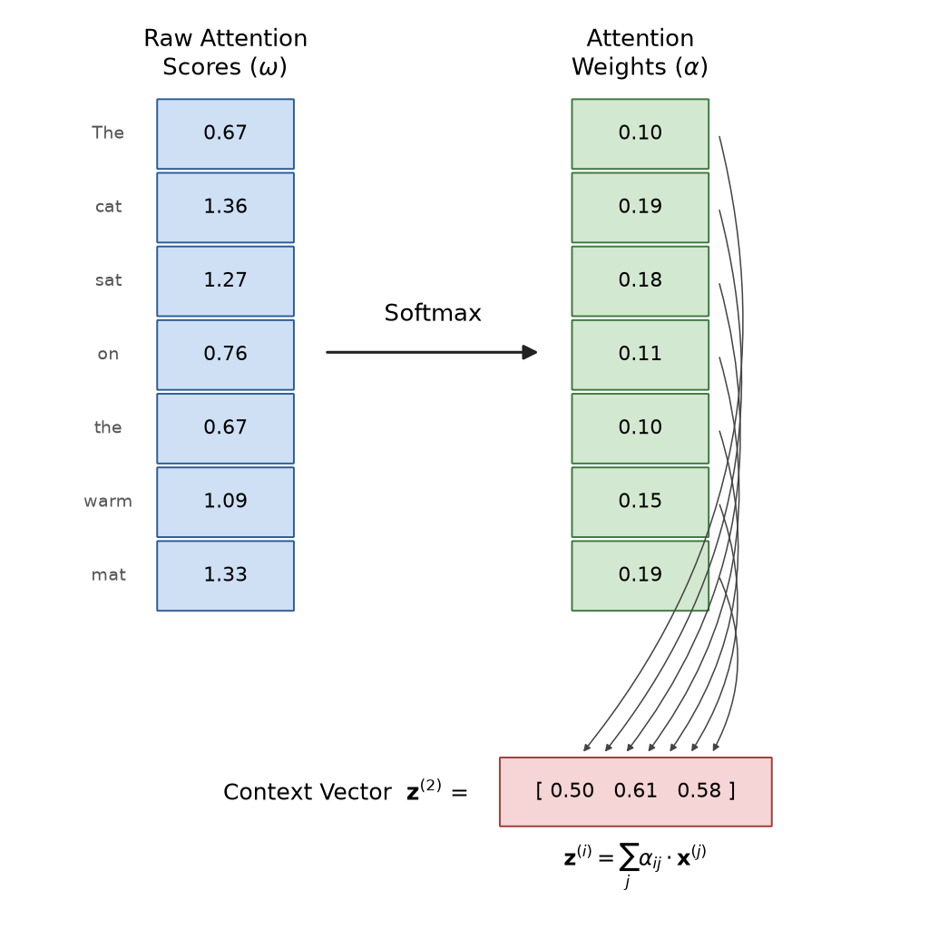
These are now our attention weights $\alpha_{2j}$ for the query token “cat”:
| Token | Raw Score ($\omega$) | Attention Weight ($\alpha$) |
|---|---|---|
| The | 0.6682 | 0.0962 (9.6%) |
| cat | 1.3581 | 0.1919 (19.2%) |
| sat | 1.2746 | 0.1765 (17.7%) |
| on | 0.7640 | 0.1059 (10.6%) |
| the | 0.6660 | 0.0960 (9.6%) |
| warm | 1.0855 | 0.1461 (14.6%) |
| mat | 1.3341 | 0.1873 (18.7%) |
After softmax, we can interpret these as percentages. “cat” allocates about 19.2% of its attention to itself, 18.7% to “mat”, 17.7% to “sat”, and less than 10% to each of “The” and “the”.
Why Softmax and Not Simple Normalisation?
You might ask: why not just divide each score by the sum of all scores? That would also make them sum to 1.
The answer is that simple normalisation (dividing by the sum) doesn’t handle negative values well, and it doesn’t amplify differences between scores. Softmax, thanks to the exponential function, has two key properties:
- All outputs are positive — $e^x > 0$ for all $x$
- It amplifies differences — a small difference in input scores becomes a larger difference in output weights, making the model more decisive about what to attend to
Step 5: Computing the Context Vector
Now we have attention weights that tell us how much “cat” should attend to each token. The final step is to compute the context vector — a new representation of “cat” that incorporates information from all the words it attends to.
The context vector is simply a weighted sum of all token embeddings, using the attention weights:
$$z^{(2)} = \sum_{j=1}^{T} \alpha_{2j} \cdot x^{(j)}$$
In plain English: multiply each token’s embedding by its attention weight, then add them all up.
# Computing the context vector for "cat"
# z^(2) = α_21 * x^(1) + α_22 * x^(2) + ... + α_27 * x^(7)

context_vector_2 = torch.zeros(inputs.shape[1])  # 3-dim vector

for i, x_i in enumerate(inputs):
    context_vector_2 += attn_weights_2[i] * x_i

print("Context vector for 'cat':")
print(context_vector_2)
# tensor([0.4964, 0.6149, 0.5813])
Or, more efficiently, as a single matrix operation:
# Efficient: matrix multiplication
context_vector_2 = attn_weights_2 @ inputs
print("Context vector for 'cat' (efficient):")
print(context_vector_2)
# tensor([0.4964, 0.6149, 0.5813])
What Does the Context Vector Mean?
The original embedding for “cat” was [0.58, 0.91, 0.44]. The context vector is [0.4964, 0.6149, 0.5813]. This new vector is not the same as the original embedding — it has been enriched with contextual information from the entire sentence.
Think of it this way:
- The original embedding for “cat” represents the word “cat” in isolation
- The context vector represents “cat” in the context of this specific sentence — a cat that sat, on something warm, on a mat
This is the magic of self-attention. The same word “cat” would get a different context vector in the sentence “The cat chased the mouse” versus “The cat sat on the warm mat”, because different words would receive different attention weights.
Step 6: Computing All Context Vectors at Once
So far we computed the context vector for just one query token (“cat”). In practice, self-attention computes context vectors for all tokens simultaneously. Let’s do this:
# Compute ALL attention scores (every token as query against every token)
# This gives us a 7x7 matrix
all_attn_scores = inputs @ inputs.T
print("Full attention score matrix (7x7):")
print(all_attn_scores)
tensor([[0.7154, 0.6682, 0.8762, 0.6010, 0.6950, 0.6115, 0.6952],
        [0.6682, 1.3581, 1.2746, 0.7640, 0.6660, 1.0855, 1.3341],
        [0.8762, 1.2746, 1.4786, 0.9650, 0.8670, 0.9315, 1.2656],
        [0.6010, 0.7640, 0.9650, 0.6478, 0.5930, 0.5399, 0.7634],
        [0.6950, 0.6660, 0.8670, 0.5930, 0.6758, 0.5999, 0.6906],
        [0.6115, 1.0855, 0.9315, 0.5399, 0.5999, 1.0374, 1.0870],
        [0.6952, 1.3341, 1.2656, 0.7634, 0.6906, 1.0870, 1.3155]])
# Apply softmax row-wise (each row is one query)
all_attn_weights = torch.softmax(all_attn_scores, dim=-1)
print("\nAttention weight matrix (rows sum to 1):")
print(all_attn_weights)

# Verify each row sums to 1
print(f"\nRow sums: {all_attn_weights.sum(dim=-1)}")
# Row sums: tensor([1., 1., 1., 1., 1., 1., 1.])
# Compute ALL context vectors in one shot
all_context_vectors = all_attn_weights @ inputs
print("\nAll context vectors:")
print(all_context_vectors)
print(f"\nShape: {all_context_vectors.shape}")
# Shape: torch.Size([7, 3])
# Verify: the context vector for "cat" (row index 1)
# matches what we computed earlier
print(f"\nContext vector for 'cat': {all_context_vectors[1]}")
# tensor([0.4964, 0.6149, 0.5813])
And there it is. In just three lines of code — matrix multiply, softmax, matrix multiply — we computed self-attention for the entire sequence.
Putting It All Together
Here is the complete, self-contained implementation from start to finish:
import torch

# ===== STEP 1: Tokenisation =====
sentence = "The cat sat on the warm mat"
tokens = sentence.split()
print(f"Tokens: {tokens}")
print(f"Number of tokens: {len(tokens)}\n")

# ===== STEP 2: Token Embeddings =====
# In practice, these would be learned. We use manual values here.
inputs = torch.tensor(
    [[0.41, 0.12, 0.73],  # The   (x^1)
     [0.58, 0.91, 0.44],  # cat   (x^2)
     [0.33, 0.76, 0.89],  # sat   (x^3)
     [0.15, 0.42, 0.67],  # on    (x^4)
     [0.39, 0.14, 0.71],  # the   (x^5)
     [0.82, 0.53, 0.29],  # warm  (x^6)
     [0.61, 0.85, 0.47]]  # mat   (x^7)
)
print(f"Input embeddings shape: {inputs.shape}\n")

# ===== STEP 3: Compute Attention Scores =====
# Dot product of every token with every other token
attn_scores = inputs @ inputs.T
print("Attention scores (raw dot products):")
print(attn_scores)

# ===== STEP 4: Normalise with Softmax =====
attn_weights = torch.softmax(attn_scores, dim=-1)
print("\nAttention weights (after softmax):")
print(attn_weights)

# ===== STEP 5: Compute Context Vectors =====
context_vectors = attn_weights @ inputs
print("\nContext vectors (self-attention output):")
print(context_vectors)

# ===== Show Results Per Token =====
print("\n" + "="*50)
print("SUMMARY: Original Embedding → Context Vector")
print("="*50)
for i, token in enumerate(tokens):
    print(f"\n  '{token}':")
    print(f"    Original:  {inputs[i].tolist()}")
    print(f"    Context:   {context_vectors[i].tolist()}")
The Intuition: Why Self-Attention Works
Let’s step back and think about what we just did:
- We started with static embeddings — each word has a fixed vector regardless of context
- We ended with context vectors — each word now has a vector that encodes its relationship to every other word in the sentence
This is fundamentally what makes Transformers so powerful. In a traditional word embedding (like Word2Vec), the word “bank” always has the same vector whether it appears in “river bank” or “bank account”. With self-attention, the context vector for “bank” would be completely different in each sentence because it would attend to different surrounding words.
The Three-Line Summary of Self-Attention
scores  = inputs @ inputs.T        # How related is each pair of tokens?
weights = torch.softmax(scores, -1) # Normalise to a probability distribution
output  = weights @ inputs          # Weighted combination of all tokens
That is it. Self-attention in three lines.
What We Didn’t Cover (Yet)
This post covered the simplest version of self-attention. Real Transformer models add several important extensions:
-
Query, Key, Value Projections (Q, K, V): Instead of using the raw embeddings directly, real Transformers project them through learned weight matrices to create separate Query, Key, and Value representations. This gives the model more expressive power.
-
Scaled Dot-Product Attention: The dot products are divided by $\sqrt{d_k}$ (where $d_k$ is the dimension of the key vectors) to prevent the softmax from becoming too peaked when dimensions are large:
$$\text{Attention}(Q, K, V) = \text{softmax}\left(\frac{QK^T}{\sqrt{d_k}}\right)V$$
-
Multi-Head Attention: Instead of one set of attention weights, Transformers compute multiple “heads” of attention in parallel, each learning to attend to different types of relationships (syntactic, semantic, positional, etc.).
-
Causal / Masked Attention: In autoregressive models (like GPT), each token can only attend to tokens that came before it, not after. This is implemented by masking future positions.
-
Positional Encoding: Since self-attention has no built-in notion of word order (it treats the input as a set, not a sequence), positional information is added to the embeddings.
Each of these is a worthy topic for its own blog post.
Key Takeaways
- Self-attention lets every token in a sequence look at every other token to build a context-aware representation.
- The process is: embed → compute dot-product scores → softmax normalise → weighted sum.
- The softmax function converts raw scores into a proper probability distribution (positive values that sum to 1).
- The context vector for each token is a weighted sum of all token embeddings, where the weights come from the attention scores.
- The entire mechanism can be expressed in three lines of matrix operations, making it highly parallelisable on GPUs.
- Self-attention is the reason Transformers can capture long-range dependencies — unlike RNNs, there is no information bottleneck between distant words.
Self-attention is beautifully simple in concept, yet extraordinarily powerful in practice. It is the building block that enables everything from machine translation to code generation to conversational AI.
After this, the next things to explore is Query-Key-Value projections, multi-head attention, and the full Transformer architecture. I don’t think I will ever go into any depth on those topics!